The Anti-Infinity Parade | Decoding Circuits

Decoding Circuits

Decoding is not an important part of error correction when quantum error correction is employed to protect against noise during the execution of quantum algorithms. We do all operations - logical operations, error correction and measurement of the output of the computation - on the encoded states themselves. Therefore, decoding is not required at all.

However, I might use decoding circuits later to assess if our error detection and correction operations are working correctly. Therefore, I will outline how to do decoding for stabilizer codes today.

Simple way of decoding

The simple way of decoding is to just run the encoding circuit in reverse. This will work perfectly. However, as you can compute, Gottesman showed another method that requires fewer operations, which we discuss below. Let's try the simple way first. We will first encode a random state and then decode it.

import stac
cd = stac.CommonCodes.generate_code('[[7,1,3]]')
cd.construct_encoding_circuit();

from random import random
from math import pi
circ = []
circ.append([f'rx({random()*pi})',6])
circ.append([f'rz({random()*pi})',6])
circ.append([f'rx({random()*pi})',6])

# TICK annotations will allow us to simulate 
# the circuit up to every TICK
# In the table below the second column has the
# state upto this TICK
circ.append(['TICK'] + [i for i in range(7)])

# then encode it.
circ += cd.encoding_circuit
# In the table below, the third column has the
# state upto this TICK
circ.append(['TICK'] + [i for i in range(6)])

# then decode
rev_enc_circ = cd.encoding_circuit.copy()
rev_enc_circ.reverse()
circ += rev_enc_circ
# The fourth column shows the state at this
# final point

# draw it
stac.draw_circuit(circ, output='latex')

# then simulate it
stac.simulate_circuit(circ, 
                      cd.num_physical_qubits+cd.num_logical_qubits, 
                      head=['basis', 'input state','enc state', 'dec state'])

code output

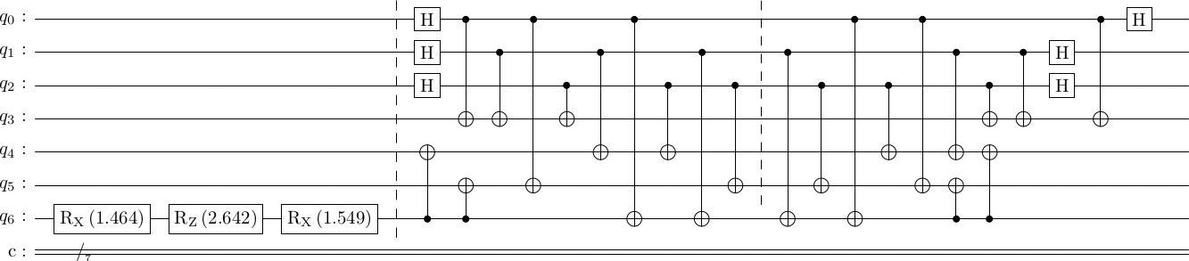
   basis  input state    enc state      dec state
--------  -------------  -------------  -------------
00000000   0.016-0.968j   0.006-0.342j   0.016-0.968j
11110000                  0.006-0.342j
01101000                 -0.015-0.087j
10011000                 -0.015-0.087j
10100100                 -0.015-0.087j
01010100                 -0.015-0.087j
11001100                  0.006-0.342j
00111100                  0.006-0.342j
00000010  -0.041-0.246j                 -0.041-0.246j
11000010                 -0.015-0.087j
00110010                 -0.015-0.087j
10101010                  0.006-0.342j
01011010                  0.006-0.342j
01100110                  0.006-0.342j
10010110                  0.006-0.342j
00001110                 -0.015-0.087j
11111110                 -0.015-0.087j

You can see that, as expected, the state decodes correctly. But, hopefully, this helps you read the table.

Gottesman's decoding algorithm

Gottesman's decoding algorithm is quite simple, and again employs the standard form of the stabilizer generator matrix that we computed last time. Instead of decoding in place, we will add $k$ (number of logical qubits) ancilla to our circuit and put the decoded state there. The steps are

Compute the standard form of the generator matrix.
Determine the logical $\bar{X}$ and logical $\bar{Z}$ operations.
Use the following algorithm to determine the decoding circuit.

decoding_circuit = []

for i in range(len(logical_zs)):
    for j in range(n):
        if logical_zs[i, n+j]:
            decoding_circuit.append(["cx", j, n+i])

for i in range(len(logical_xs)):
    for j in range(n):
        if logical_xs[i, j] and logical_xs[i, n+j]:
            decoding_circuit.append(["cz", n+i, j])
            decoding_circuit.append(["cx", n+i, j])
        elif logical_xs[i, j]:
            decoding_circuit.append(["cx", n+i, j])
        elif logical_xs[i, n+j]:
            decoding_circuit.append(["cz", n+i, j])

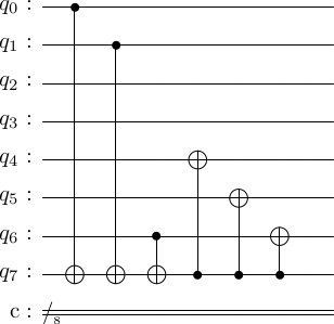
As you can see, this algorithm just reads off the entries of the logical operators, and applies appropriate control operations to and from the ancilla qubits. You can refer to Frank Gaitan's book [1] if you want the detailed reasoning for why this algorithm indeed works.

Exercise: Determine the number of operations required for Gottesman's encoding algorithm. What is the depth of the circuit? Determine the number of operations required for Gottesman's decoding algorithm. What is the depth of the circuit?

Now, let's try this.

cd.standard_form()
print("G =")
stac.print_matrix(cd.standard_gens_mat, augmented=True)
cd.construct_logical_operators()
print("Logical X =")
stac.print_matrix(cd.logical_xs, augmented=True)
print("Logical Z =")
stac.print_matrix(cd.logical_zs, augmented=True)

dec_circ = cd.construct_decoding_circuit()

stac.draw_circuit(dec_circ, output='latex')

G =

$\displaystyle \left(\begin{array}{ccccccc|ccccccc} 1 & 0 & 0 & 1 & 0 & 1 & 1 & 0 & 0 & 0 & 0 & 0 & 0 & 0 \\ 0 & 1 & 0 & 1 & 1 & 0 & 1 & 0 & 0 & 0 & 0 & 0 & 0 & 0 \\ 0 & 0 & 1 & 1 & 1 & 1 & 0 & 0 & 0 & 0 & 0 & 0 & 0 & 0 \\ 0 & 0 & 0 & 0 & 0 & 0 & 0 & 1 & 1 & 1 & 1 & 0 & 0 & 0 \\ 0 & 0 & 0 & 0 & 0 & 0 & 0 & 1 & 0 & 1 & 0 & 1 & 0 & 1 \\ 0 & 0 & 0 & 0 & 0 & 0 & 0 & 0 & 1 & 1 & 0 & 0 & 1 & 1 \\ \end{array}\right)$

Logical X =

$\displaystyle \left(\begin{array}{ccccccc|ccccccc} 0 & 0 & 0 & 0 & 1 & 1 & 1 & 0 & 0 & 0 & 0 & 0 & 0 & 0 \\ \end{array}\right)$

Logical Z =

$\displaystyle \left(\begin{array}{ccccccc|ccccccc} 0 & 0 & 0 & 0 & 0 & 0 & 0 & 1 & 1 & 0 & 0 & 0 & 0 & 1 \\ \end{array}\right)$

code output

Does this actually work? Let's try. It will be a bit difficult to see the working of this algorithm with random states, so let's work with the basis states. First, we will see if the zero state is decoded properly.

cd.construct_encoding_circuit()

# first create the zero state
circ = []
circ.append(['TICK'] + [i for i in range(7)])

# then encode it.
circ += cd.encoding_circuit
circ.append(['TICK'] + [i for i in range(6)])

# then decode
circ += cd.decoding_circuit

stac.draw_circuit(circ, output='latex')
stac.simulate_circuit(circ, 
                      cd.num_physical_qubits+cd.num_logical_qubits, 
                      head=['basis', 'input state','enc state', 'dec state'])

code output

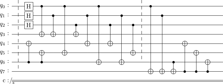
   basis  input state      enc state    dec state
--------  -------------  -----------  -----------
00000000   1.000               0.354        0.354
11110000                       0.354        0.354
11001100                       0.354        0.354
00111100                       0.354        0.354
10101010                       0.354        0.354
01011010                       0.354        0.354
01100110                       0.354        0.354
10010110                       0.354        0.354

The input state here is the $7$ th qubit counting from the left, out of the $8$ qubits. The first $6$ qubits are the encoding ancilla, and the last qubit is the decoding ancilla.

You can see that the input state is $\ket{0000000}\ket{0}$ . Then, we apply the encoding operation to get the encoded $\ket{\bar 0}$ state. After decoding, note that the state of the $8$ th qubit is still $0$ . This is not very interesting now. But, let's try with the one state.

# first create the one state
circ = []
circ.append(['x',6])
circ.append(['TICK'] + [i for i in range(7)])

# then encode it.
circ += cd.encoding_circuit
circ.append(['TICK'] + [i for i in range(6)])

# then decode
circ += cd.decoding_circuit

stac.draw_circuit(circ, output='latex')
stac.simulate_circuit(circ, 
                      cd.num_physical_qubits+cd.num_logical_qubits, 
                      head=['basis', 'input state','enc state', 'dec state'])

code output

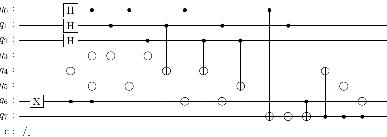
   basis  input state    enc state    dec state
--------  -------------  -----------  -----------
01101000                  0.354
10011000                  0.354
10100100                  0.354
01010100                  0.354
00000010   1.000
11000010                  0.354
00110010                  0.354
00001110                  0.354
11111110                  0.354
00000001                               0.354
11110001                               0.354
11001101                               0.354
00111101                               0.354
10101011                               0.354
01011011                               0.354
01100111                               0.354
10010111                               0.354

And voila, you see that in the final state, the $8$ th qubit is in the state $\ket{1}$ , hence unentangled from the remaining qubits. Also, note that the state of the first $7$ qubits has changed into something outside the logical code space (none of the kets that appear in the logical zero and one states are here). This ensures that the first $7$ qubits no longer contain any information about an arbitrary logical qubit, hence, respecting the no-cloning theorem.

Fun with quirk

Finally, stac has a handy function to convert circuits to Quirk. Copy and paste the following url into your browser to make it go.

stac.circuit_to_quirk(circ)

https://algassert.com/quirk#circuit={"cols":[[1, 1, 1, 1, 1, 1, "X", 1], [1, 1, 1, 1, "X", 1, "•", 1], [1, 1, 1, 1, 1, "X", "•", 1], ["H", 1, 1, 1, 1, 1, 1, 1], ["•", 1, 1, "X", 1, 1, 1, 1], ["•", 1, 1, 1, 1, "X", 1, 1], ["•", 1, 1, 1, 1, 1, "X", 1], [1, "H", 1, 1, 1, 1, 1, 1], [1, "•", 1, "X", 1, 1, 1, 1], [1, "•", 1, 1, "X", 1, 1, 1], [1, "•", 1, 1, 1, 1, "X", 1], [1, 1, "H", 1, 1, 1, 1, 1], [1, 1, "•", "X", 1, 1, 1, 1], [1, 1, "•", 1, "X", 1, 1, 1], [1, 1, "•", 1, 1, "X", 1, 1], ["•", 1, 1, 1, 1, 1, 1, "X"], [1, "•", 1, 1, 1, 1, 1, "X"], [1, 1, 1, 1, 1, 1, "•", "X"], [1, 1, 1, 1, "X", 1, 1, "•"], [1, 1, 1, 1, 1, "X", 1, "•"], [1, 1, 1, 1, 1, 1, "X", "•"]]}

[1] Gaitan, Frank, Quantum Error Correction and Fault Tolerant Quantum Computing (CRC Press, 2008).

Oct 13, 2022

Decoding Circuits

Simple way of decoding

Gottesman's decoding algorithm

Fun with quirk