Syndrome Measurements
The critical part of any error correcting code is error-detection. For the stabilizer codes in general, error-detection is done by measuring each of the stabilizer generators on the state. An error-free state is a eigenstate of all stabilizer generators, and will lead to all measurement results . On the other hand, non-trivial errors anti-commute with one or more generators, which means that any corrupted state is a eigenstate of some generators. Measurements reveal these, and we can then infer which error occured. For a simple code like the Steane code, this is quite simple and can be done exactly. However, once we concatenate the code into a larger code so we can correct more errors, things become more dicey and we can only guess which error occured with some probability. But that is a discussion for another time.
Right now, let's figure out how to measure the stabilizer generators. I will three ways of doing these syndrome measurements for the Steane code.
- Straightforward measurements using a single ancilla per generator. This is not fault-tolerant. We will see how a single error will lead to multiple errors in the logical state.
- A fault-tolerant method using the cat state.
- A fault-tolerant method using the Shor state.
Preliminary: Non-destructive measurements
Before, we get started on the measurement of the generators, we need to figure out how to do non-destructive measurements using quantum circuits. It is quite important that we do non-destructive measurements on the encoded qubits, so we don't destroy any superpositions, , that the encoded qubits are in. Thankfully, we are only interested in a gaining a small amount of information about the state; whether it is in the codespace or in one of the corrupted code spaces. This information is not at all related to the superposition the logical qubits are in, so we can extract the required information with non-destructive measurements.
How do we do this? Suppose, we want to do an measurement on a single-qubit in state . What is the expected result?
| measurement outcome | probability | post measure state of qubit 0 |
|---|---|---|
| 0 | ||
| 1 |
This is done as follows, where the th qubit is the one being meaesured, and the st qubit in an ancilla.
import stac
circ = stac.Circuit()
circ.append('H', 1)
circ.append('CZ', 1, 0)
circ.append('H', 1)
circ.append('MR', 1)
circ.draw()
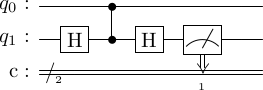
Let's work our way through this circuit. First, the input state under the goes to . Then the results in, . Next, the sends the state to
At this point, if we measure the ancilla, then the outcomes are
| measurement outcome | probability | post-measure state of qubit 0 |
|---|---|---|
| 0 | $ | \alpha |
| 1 | $ | \beta |
As we can see, this is what we wanted.
Does this process work in general? I.e. if we want to measure operator , we do a instead of a in the circuit above? This is quite simple to show. We know that the state at the end of the circuit will be
Let have an eigenbasis . Then, if we expand , then, the algebra is the same, and we get , and measurements of the ancilla indeed measures qubit 0 in the basis.
Does this process work if we want to measure a multi-qubit state, using a multi-qubit Pauli operator? Yes. Recall that every element in the Pauli group only has two eigenvalues . So, our analysis will continue to hold, with the measurement outcome on the ancilla is the measurement of the unknown qubit state, and the measurement.
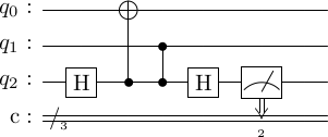
So, to measure, say , we would implement the circuit below.
circ = stac.Circuit()
circ.append('H', 2)
circ.append('CX', 2, 0)
circ.append('CZ', 2, 1)
circ.append('H', 2)
circ.append('MR', 2)
circ.draw()
Measurement of stabilizer generators
One of the features of the measurement process described is that measuring an arbitrary operator on a state will destroy the superposition of the state (as governed by the rules of quantum mechanics). However, quantum stabilizer codes avoid this possibility. To see this, suppose that we want to measure the generator . This generator has the properties that, if is the encoded state, then and Then, at the end of the measurement circuit, the qubits will be in state where for some arbitrary error .
- If , then .
- If , then .
This is because either vanishes or vanishes depending on whether is the corrupted state or the uncorrupted state. This happens because the logical state is stabilized by the very generator we are trying to measure.
To summarize, if there is
- no error, then measuring ancilla will yield ,
- an error, then measuring ancilla will yield .
Syndrome measurements for the Steane code
We can now figure out the measurement of the stabilizers of the Steane code. The canonical generators are as follows.
cd = stac.CommonCodes.generate_code("[[7,1,3]]")
stac.print_matrix(cd.gens_mat, augmented=True)
From these, constructing the measurements is quite simple.
for i in range(num_generators):
    self.syndrome_circuit.append(["h", n+i])

for i in range(num_generators):
    for j in range(num_physical_qubits):
        if gens_x[i, j] and gens_z[i, j]:
            syndrome_circuit.append(["cx", n+i, j])
            syndrome_circuit.append(["cz", n+i, j])
        elif gens_x[i, j]:
            syndrome_circuit.append(["cx", n+i, j])
        elif gens_z[i, j]:
            syndrome_circuit.append(["cz", n+i, j])

for i in range(self.num_generators):
    syndrome_circuit.append(["h", n+i])

for i in range(num_generators):
        syndrome_circuit.append(['MR', self.num_physical_qubits+i])
cd.construct_syndrome_circuit();
cd.syndrome_circuit.draw()
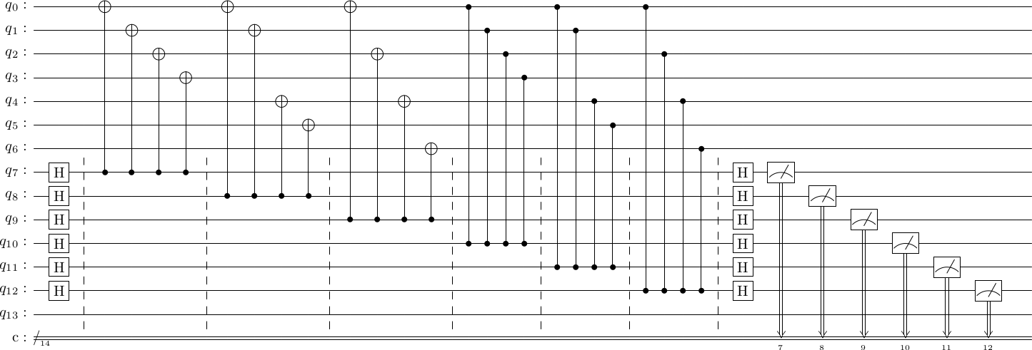
To use this in practice, we will
- Encode the zero state
- Introduce an error
- Measure the stabilizers
# Step 1
circ = cd.construct_encoding_circuit()
circ.append('TICK', 0, cd.num_physical_qubits+cd.num_generators)

# Step 2
circ.append('X', 2)

# Step 3
circ += cd.syndrome_circuit

circ.draw()

# we use stim to simulate this circuit
import stim
stim_circ = stim.Circuit(circ.stim())
sample = stim_circ.compile_sampler().sample(1)[0]
print(1*sample)
[0 0 0 1 0 1]
As we can see, an error on the 2nd qubit leads to a the 3rd and 5th generators failing (counting from 0). The syndrome vector is the th column (counting from 1) of the generator matrix, because as discussed previously it is the -type stabilizer generators that detect bit-flip errors. In this way, each of the -type errors and -type errors correspond to one of the columns of the generator matrix.
Vulnerability of this code to errors
Within any error-correcting code, the coupling of ancilla blocks can possibly increase the number of errors. This is a problem, and we need to design methods of measuring the syndromes that minimizes additional errors. Principally, there are two bad things that can happen
- An error occurs in the ancilla block and propogates to multiple code block qubits. (recall our definition of fault-tolerance where a single error in one block should create no more than one error in another block).
- A single error on the logical block propogates down to the ancilla and then propogates back up to another logical qubit. This will not actually happen, but we should check.
Here, we analyze each of these cases. To make the dicussion concrete, I am going to draw the syndrome measurement circuit again, and mark the locations where error could occur.
circ = cd.construct_encoding_circuit()
circ.append('TICK', 0, cd.num_physical_qubits-1)
circ.insert_errors(before_op="end", error_types=["E"])
circ.append('TICK', 0, cd.num_physical_qubits+cd.num_generators-1)
cd.construct_syndrome_circuit()
cd.syndrome_circuit.insert_errors(before_op="CX", error_types=["E", "I"])
cd.syndrome_circuit.insert_errors(before_op="CZ", error_types=["E", "I"])
circ += cd.syndrome_circuit
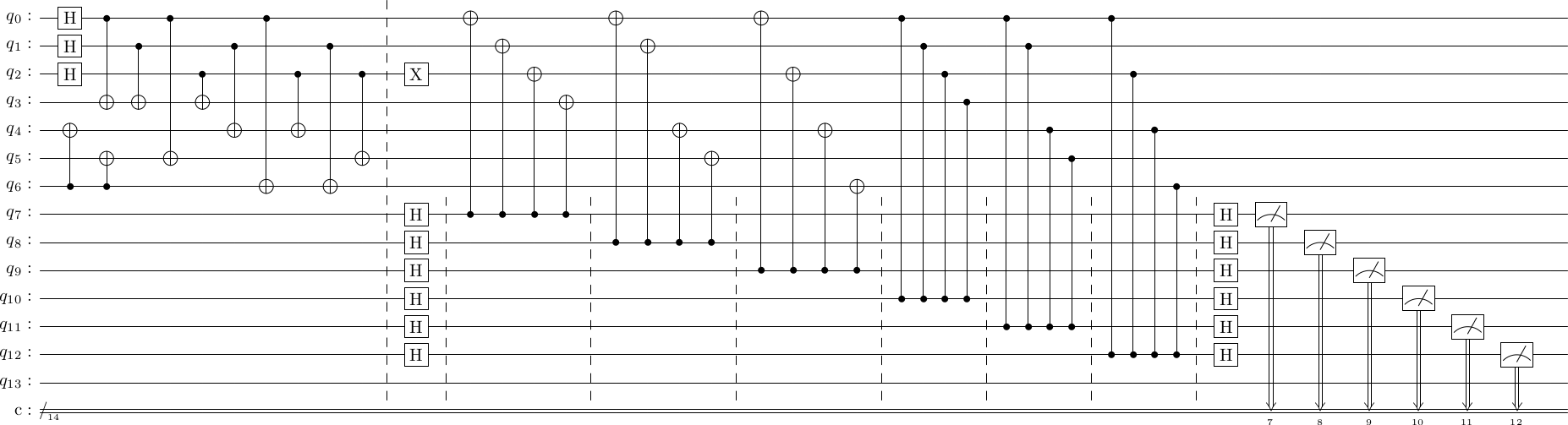
circ.draw()
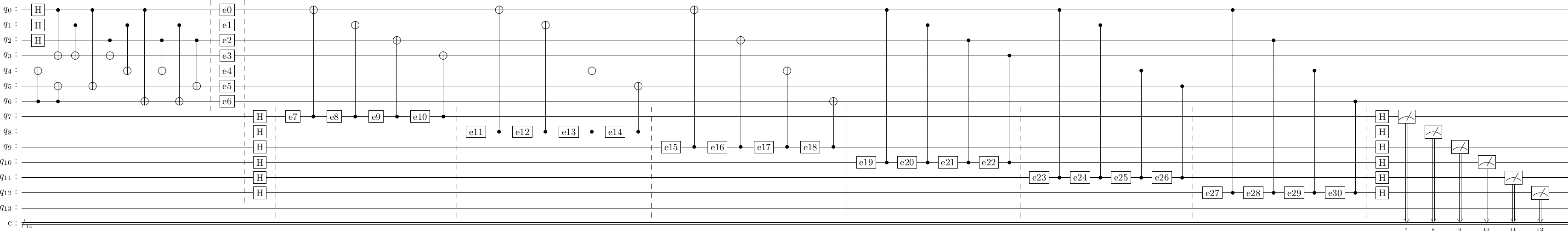
In the picture above (please right-click and open the image to see a larger version), I have annoted and numbered all the locations where an "interesting" error could occur. The uninteresting places are
- Errors within the initial encoding part, which won't allow the code even a fighting chance. We will relax this assumption later, when we study fault-tolerant ways of encoding.
- On the ancilla qubits, there are no errors before the Hadamard gates. This is because an error directly before the Hadamard is equal to its Hadamard conjugate after the Hadamard, e.g. . And we already have gates right after the Hadamard.
- There are no errors directly before the final measurements because their effect is obvious: an incorrect syndrome measurement.
- For the same reason as the second point, there are no errors right before the final Hadamard gates.
- Errors could occur on the code qubits at any point, but because they are all target qubits, an error at one point is equivalent to another point.
To check the impact of various sets of these errors, we first need to remind ourselves of some more conjugacy relations.
Conjugacy relations
Conjugacy relations allow us to build equivalent circuits. For instance, we can compute directly that , so these are two equivalent circuits. This same equation can be rewritten as . So computing the left hand side tells us what gate moving the past creates. Relations needed are
We are now ready to analyze the effects of various errors. Our method of analysis will be to use the conjugacy relations to move the error through the circuit and see if other qubits are affected.
Error on code qubits e0-e6
A circuit that shows how these errors will interact with the ancilla qubits is as follows, where the first 4 qubits are a subset of the code qubits, and the last qubit is one of the ancilla. First, we analyze the case of the gates in the syndrome measurements. We show the generic error 'e0'.
circ = stac.Circuit()
stac.Circuit.error_ind = 0
circ.append_error(0)
circ.append('TICK',0,4)
circ.append('H', 4)
for i in range(4):
    circ.append('CX', 4, i)
circ.append('H', 4)
circ.draw()

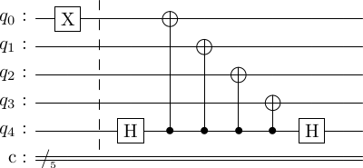
- Now, suppose e0 = . As we can see from the conjugacy table, if is on the target qubit of , then it commutes past the . No other qubit is effected. In other words, the two circuits below are equivalent.
circ = stac.Circuit()
circ.append('X',0)
circ.append('TICK',0,4)
circ.append('H', 4)
for i in range(4):
circ.append('CX', 4, i)
circ.append('H', 4)
circ.draw()
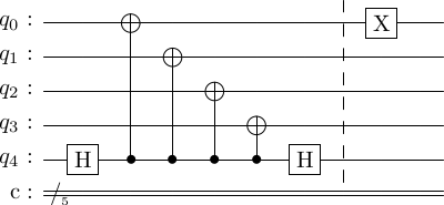
circ = stac.Circuit()
circ.append('H', 4)
for i in range(4):
circ.append('CX', 4, i)
circ.append('H', 4)
circ.append('TICK',0,4)
circ.append('X',0)
circ.draw()
This means is that an error of type e0-e6 does not propogate to any other qubit via the gates. This is expected, as the stabilizer measurement of this nature is not designed to detect errors.
- Now, suppose the e0 = . From the conjugacy table, we see that the . In other words, we have the two equivalent circuits.
circ = stac.Circuit()
circ.append('Z',0)
circ.append('H', 4)
for i in range(4):
    circ.append('CX', 4, i)
circ.append('H', 4)
circ.draw()

circ = stac.Circuit()
circ.append('H', 4)
circ.append('CX', 4, 0)
circ.append('Z', 0)
circ.append('Z', 4)
for i in range(1, 4):
    circ.append('CX', 4, i)
circ.append('H', 4)

circ.draw()
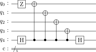
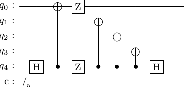
At this point, can no longer propogate to any other qubit, but can ? From the conjugacy relations, we see that . In this way, we can move through all the gates and past the to get.
circ = stac.Circuit()
circ.append('H', 4)
for i in range(4):
    circ.append('CX', 4, i)
circ.append('H', 4)
circ.append('Z',0)
circ.append('X',4)
circ.draw()
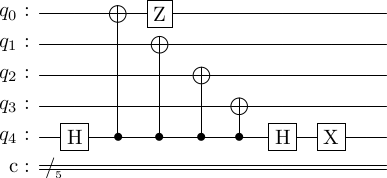
In particular, once the error has moved down to the ancilla qubits (which it should so we can detect it), it no longer propogates back up to the code qubits. The final state of the ancilla is , which indicates the detected error.
Exercise. Repeat the above analysis for the -type stabilizer measurements.
Error e7, e11, e15
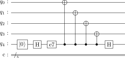
Error e7 confused me for a bit when I first analyzed it initially. It seems like it can cause problems, but it does not. In the circuit below, I have not only drawn e7, but also shown that the ancilla qubits are initialized to at the start of the circuit.
circ = stac.Circuit()
stac.Circuit.error_ind = 7
circ.append('R', 4)
circ.append('H', 4)
circ.append_error(4)
for i in range(4):
    circ.append('CX', 4, i)
circ.append('H', 4)
circ.draw()
-
Now, suppose that e7 = . Does this effect the state of the ancilla qubit? No, it does not. The ancilla qubit is in state just before the error occurs, and the . So this error doesn't change anything. This is fortunate, because the conjugacy relations tell us that an on the control qubit propagates up to the target qubit as well. But this is avoided by the state the ancilla is in.
-
Now, suppose that e7 = . This changes the state of the ancilla to . So something bad will happen. If you run through the calculations we did above, you will note that if the ancilla is in $\ket{-}, then we get the opposite syndrome to what we think corresponds to an error. So, even if there is no error on the code qubits, we will think there is due to this error.
But does the error propagate to the code qubits. The answer is no, as we have already discussed. gates on the control qubit do not propogate to the target qubit of .
Exercise. Repeat the above analysis for the impact of e19, e23, e27 on the gates.
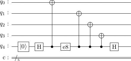
Error e8, e9, e10, etc
These are the nasty errors and can cause lots of problems. To fully, understand this, let's do some calculations. The error free circuit is as follows.
circ = stac.Circuit()
circ.append('R', 4)
circ.append('H', 4)
for i in range(4):
    circ.append('CX', 4, i)
circ.append('H', 4)
circ.draw()
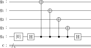
Let the code qubits be in state . The the circuit propagation is as follows. transforms under to . Then the three control gates only trigger for the second term, and we get We don't evaluate the effect of the final .
Now, let's put in the error.
circ = stac.Circuit()
stac.Circuit.error_ind = 8
circ.append('R', 4)
circ.append('H', 4)
circ.append('CX', 4, 0)
circ.append_error(4)
for i in range(1, 4):
    circ.append('CX', 4, i)
circ.append('H', 4)
circ.draw()
-
Suppose that e8 = . Then, the circuit propagation is as follows. goes to under the first . Then, the first transforms it to Now, the error takes the state to The remaining control gates now trigger on the first term
As you can see, this state is quite different from the error-free circuit state. This is unlike the case of e7. Why is that? e7 occurs before the ancilla is entangled with the code qubits. Hence, the gates stabilizes the unentangled state in the case of e7 = . Here, the error occurs after the ancilla is entangled, so the error can no longer stabilize the ancilla.
It should be clear from the above that a single error on the ancilla has caused an error on not just the ancilla, but on three of the code qubits. To see this in an alternate fashion, note from the conjugacy relations that . So the subsequent control gates propogate the error to the code qubits , and .
Finally note that the syndrome in this case will be widely wrong, as the syndromes correspond to one single-qubit error and here we have three single-qubit errors.
-
Suppose that e8 = . By similar calculations, we get This is only an error on the ancilla, and will result in the wrong syndrome.
Exercise: Repeat this analysis for the -type measurements.
Analysis summary and fault-tolerance
Our analysis of the -type measurements have yielded the following results.
| Error representative | Error type | Code qubits errors | Syndrome correct? |
|---|---|---|---|
| e0 | X | 1 | Yes |
| e0 | Z | 1 | Yes |
| e7 | X | 0 | Yes |
| e7 | Z | 0 | No |
| e8 | X | 3 | No |
| e8 | Z | 0 | No |
As we can see, there exists errors on the ancilla qubits that create multiple errors on the code qubits. This is problematic, and does not match our requirements for fault-tolerant quantum computing.
Next time, we will discuss fault-tolerant methods of stabilizer measurements.