Algorithms for code concatenation

My goal is to compute fault-tolerance thresholds for stabililzer codes. To this end, we need to understand how to concatenate quantum codes. Briefly, code concatenation is when a state is encoded first by one code, then the encoded qubits again by same or another code. The resultant qubits may be encoded again by another code, and so on. The entire concatenation of codes can be treated as a single code, which has a larger number of physical qubits than any of the individual codes but also a larger a distance.

In our study of code concatenation, we are interested in the following:

• What are the generators of the concatenated code?
• How to perform encoding and logical operations of the code?
• How to do error correction.

Today, I will be mostly interested in the first question. My development will follow the algorithms presented by Gaitan [1], though I have made significant advances in the clarity of the arguments.

First foray: a two layer concatenation

Suppose, we encode $k_1$ qubits using the code $C_1 \sim [[n_1,k_1,d_1]]$. This yields $n_1$ encoded qubits. We then take each of these qubits, and encode each one separately using $C_2 \sim [[n_2, k_2 = 1, d_2]]$. We will refer to the concatenated code as $C = C_2 \circ C_1$.

This process can be visualized as follows. The numbers indicate how many elements are in the box to their right.

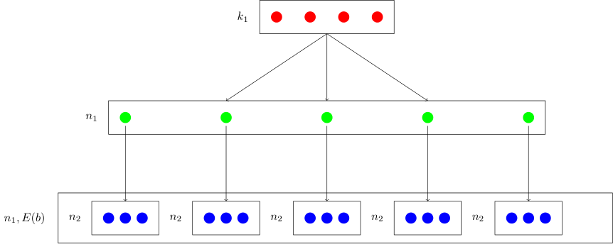
Let's first consider the question of generators. The generators of $C_1$ are $\{g_i^1, i=0,\dots,n_1-k_1-1\}$ and $C_2$ are $\{g_i^2, i=0,\dots,n_2-2\}$. What are the generators of $C$? To answer this, let $\ket{\psi}_{k_1}$ be a state of $k_1$ qubits that is to be encoded. The first encoding is written as $$\ket{\psi}_{k_1} \stackrel{C_1}{\to} \ket{\bar\psi}_{n_1}.$$ We note for now that for all $i$, $$g_i^1\ket{\bar\psi} = \ket{\bar\psi}.$$

Now, for the second round of encoding, we will separate each of the $n_1$ qubits and encode each one using $C_1$. To write this, let $\lambda = (\lambda_0, \lambda_1,\dots, \lambda_{n_1-1})$. Then $$\ket{\bar\psi} = \sum_{\lambda_i = 0,1} \alpha_\lambda \ket{\lambda_0}_1 \otimes \ket{\lambda_1}_1 \otimes \cdots \otimes \ket{\lambda_{n_1-1}}_1.$$ When we encode each qubit, we obtain, $$\ket{\bar\psi} \stackrel{C_2}{\to} \ket{\bar{\bar\psi}} = \sum_{\lambda_i = 0,1} \alpha_\lambda \ket{\bar\lambda_0}_{n_2} \otimes \ket{\bar\lambda_1}_{n_2} \otimes \cdots \otimes \ket{\bar\lambda_{n_1-1}}_{n_2},$$ where the bars in $\ket{\bar\lambda_i}_{n_2}$ indicate that it is an encoded state, and the subscript indicates that it has $n_2$ qubits. To summarize, let us call each block of $n_2$ qubits $E(b)$, where $b=0,\dots,n_1-1$ because there are $n_1$ such blocks.

Generators

In this way, our doubly encoded state is a $n_1n_2$ qubit state. Overall, we have encoded $k_1$ qubits into $n=n_1n_2$ qubits. This means that the concatenated code must have $n_1n_2-k_1$ generators. Let's find them.

(1) Consider a generator $g^2_l$ of $C_2$, which is a $n_2$ qubit operator, but we have to be careful over which qubits it acts. For instance, we can write $g^2_l \otimes I_{n-n_2}$ to obtain an operator that acts on the first $n_2$ qubits of $n$ total qubits. Similarly, we can write $I_{n_2} \otimes g^2_l \otimes I_{n-2n_2}$ to obtain an operator that acts on the next $n_2$ qubits. This notation will get tedious fast, so let's just write $g^2_l[i,j]$ to indicate that $g^2_l$ acts on qubits $i, i+1, \dots, j-1$, where $j-i = n_2$.

Now, it's quite easy to see from definition that for all $i$, $$g^2_l[n_2 i, n_2 (i+1)] \ket{\bar\lambda_i}_{n_2} = \ket{\bar\lambda_i}_{n_2},$$ i.e. if $g^2_l$ is made to act on the $i$-th block of $n_2$ qubits in the final block, it will be a stabilizer operation. In other words, we have discovered that the set $\{g^2_l[n_2 i, n_2(i+1)], l=0,\dots,n_2-2, i=0, \dots, n_1-1\}$ stabilizes the state $\ket{\bar{\bar\psi}}$. We can count that there are $n_1(n_2-1)$ such operators.

(2) But wait, there are more operators that stabilize the state $\ket{\bar{\bar\psi}}$. Let $\xi_2$ be the encoding operation for $C_2$. Then $\xi_2^{\otimes n_1}$ is the encoding operations for the second step. Conversely, $\left(\xi_2^{\otimes n_1}\right)^\dagger$ is the decoding operation. Then, $\left(\xi_2^{\otimes n_1}\right)^\dagger\ket{\bar{\bar\psi}} = \ket{\bar\psi}$. We noted earlier that $g^1_l$ stabilizes this state. Hence, $$\xi_2^{\otimes n_1}g^1_l\left(\xi_2^{\otimes n_1}\right)^\dagger\ket{\bar{\bar\psi}} = \ket{\bar{\bar\psi}}.$$

Hence, the set $\{\xi_2^{\otimes n_1}g^1_l\left(\xi_2^{\otimes n_1}\right)^\dagger, l = 0, \dots, n_1-k_1-1\}$ must also stabilize the doubly encoded state. There are $n_1-k_1$ such operators.

In total, we have $n_1(n_2-1) + (n_1-k_1) = n_1n_2-k_1$ stabilizers. As we have found sufficient number of stabilizers, we are done.

How to put this mathematics into practice

Let's try to construct the algorithm that creates the generators of the concatenated code. We will depend on the vector representation of the Pauli operators.

(1) Constructing the first set of generators is very simple. We just have to do some shifting. Note that $g^2_l$, an operator on $n_2$ qubits, is represented by a vector of length $2n_2$. We have to construct, $g^2_l[n_2 i, n_2(i+1)]$, an operator over $n$ qubits, which is represented by a vector of length $2n$. The code is right there is the notation.

Call $g=g^2_l$. Then

# for each of the E(b) blocks
for b in range(n_1):
    for each g:
        encoded_g = zeros((1,2*n))
        # for the X part
        encoded_g[n_2*b: n_2*(b+1)] = g[:n2]
        # for the Z part
        encoded_g[n + n_2*b: n + n_2*(b+1)] = g[n2:]

(2) For the second set, we have to do a little bit of work to understand encoding. If we use $C_2$ to encode a qubit, it takes the logical operators $X, Z$ of the qubit and maps them to the encoded $\bar{X} = \xi_2X\xi_2^\dagger, \bar{Z} = \xi_2 X\xi_2^\dagger$. In vector notation, $X=(1|0)$ and $Z=(0|1)$ and these are mapped to vectors of length $2n_2$. This mapping is already known and we have constructed it before.

Now, we have $g^1_l$ which is an operator over $n_1$ qubits, which means it is the product of $n_1$ different Pauli operators, i.e. $g^1_l = P_0 \otimes P_1 \otimes \cdots \otimes P_{n_1-1}$. It is represented by a vector of length $2n_1$. So $$\{\xi_2^{\otimes n_1}g^1_l\left(\xi_2^{\otimes n_1}\right)^\dagger = \xi_2P_0\xi_2^\dagger \otimes \xi_2P_1\xi_2^\dagger \otimes \cdots \otimes \xi_2P_{n_1-1}\xi_2^\dagger.$$ Our algorithm is now clear. We iterate over the operators in $g=g^1_l$ and encode each according to the mapping $\bar{X} = \xi_2X\xi_2^\dagger, \bar{Z} = \xi_2 X\xi_2^\dagger$. We have to be careful about the shifting as before, because $\xi_2P_i\xi_2^\dagger$ acts on qubits $n_2 i$ to $n_2 (i+1) - 1$.

# declare
# logical_x
# logical_z
for each g:
    encoded_g = zeros((1,2*n_1*n_2))
    for i in range(n1):
        if g[i] and g[n+i]: #P_i is the Y operator
            # multipling operators corresponds to adding their vectors mod 2
            encoded_g[n2*i: n2*(i+1)] += logical_x[:n2] + logical_z[:n2]
            encoded_g[n + n2*i: n + n2*(i+1)] += logical_x[n2:] + logical_z[n2:]
        elif g[i]: # P_i is the X operator
            encoded_g[n2*i: n2*(i+1)] += logical_x[:n2]
            encoded_g[n + n2*i: n + n2*(i+1)] += logical_x[n2:]
        elif g[n+i] # P_i is the Z operator
            encoded_g[n2*i: n2*(i+1)] += logical_z[:n2]
            encoded_g[n + n2*i: n + n2*(i+1)] += logical_z[n2:]    

That wasn't too difficult.

$k_2$ does not have to be $1$, but $k_2$ divides $n_1$

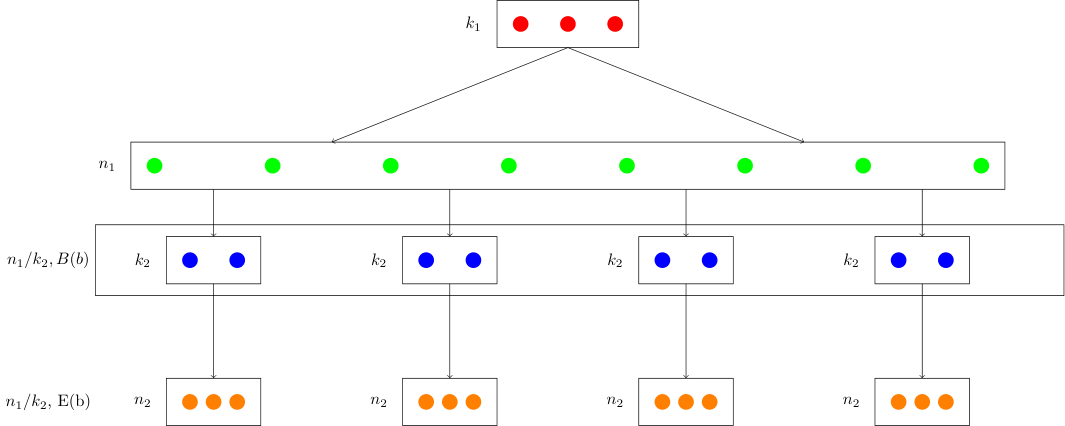
Let us now relax the assumption that $k_2=1$, but let it be an interger that divides $n_1$. This will complicate the encoding in the second round. As before, the first round is $$\ket{\psi}_{k_1} \stackrel{C_1}{\to} \ket{\bar\psi}_{n_1}.$$ Because $n_1$ is divisible by $k_2$, these $n_1$ qubits can be divided into $n_1/k_2$ blocks, each of size $k_2$. Let the blocks of qubits be called $B(b)$ for $b=0,\dots,n_1/k_2-1$. Let $\gamma = (\gamma_0,\dots,\gamma_{n_1/k_1-1})$, and let $B$ be the basis of a $2^{k_2}$ dimensional Hilbert space. We can write the first-round encoded state as $$\ket{\bar\psi}_{n_1} = \sum_{\ket{\gamma_i}\in B} \alpha_\gamma \ket{\gamma_0}_{k_2} \otimes \ket{\gamma_1}_{k_2} \otimes \cdots \otimes \ket{\gamma_{n_1/k_2 - 1}}_{k_2},$$ broken up into a sum over $k_2$-qubit basis states.

Now, we encode each block using $C_2$, to create a new encoded block $E(b)$ of size $n_2$. This creates the final state $$\ket{\bar\psi}_{n_1} \stackrel{C_2}{\to}\ket{\bar{\bar\psi}} = \sum_{\ket{\gamma_i}\in B} \alpha_\gamma \ket{\bar\gamma_0}_{n_2} \otimes \ket{\bar\gamma_1}_{n_2} \otimes \cdots \otimes \ket{\bar\gamma_{n_1/k_2 - 1}}_{n_2}.$$ This final state has $n_1/k_2$ blocks each of size $n_2$ qubits, for a total of $n = n_1n_2/k_2$ qubits. Hence, in this code $k_1$ qubits are encoded to $n_1n_2/k_2$ qubits, which is fewer than before.

The structure of the generators is similar to what we had above.

(1) If we apply the operator $g^2_l$ to the $b$-th encoded block $E(b)$, when the qubits are in state $\ket{\bar{\bar\psi}}$ we find that it stabilizes the state. Hence, it must be a stabilizer of the doubly encoded state. As before the $n_2$ sized operator $g^2_l$ when acting on the $b$-th block is labelled $g^2_l[n_2 * b, n_2 * (b+1)]$. It's algorithmic implementation is as before, except the change in the number of blocks $E(b)$.

(2) What about the $g^1_l$ associated generators? Things are a bit more convoluted because of the grouping of the qubits. Now, note that $\xi_2$ is an operator that takes $k_2$ qubits to $n_2$ qubits, and in the second encoding, we apply $\xi_2$ to each group $B(b)$ of qubits. This means that $$\xi_2^{\otimes n_1/k_2}\ket{\bar\psi} = \ket{\bar{\bar\psi}}.$$ Hence, our stabilizers are given by $$\xi_2^{\otimes n_1/k_2}g^1_l\left(\xi_2^{\otimes n_1/k_2}\right)^\dagger\ket{\bar{\bar\psi}} = \ket{\bar{\bar\psi}}.$$

How do we process $\xi_2^{\otimes n_1/k_2}g^1_l\left(\xi_2^{\otimes n_1/k_2}\right)^\dagger$? If, as before, $g^1_l = P_0 \otimes P_1\otimes \cdots \otimes P_{n_1}$, then we break it up according to $B(b)$ into chunks of $k_2$, to form $$g^1_l = (P_0 \otimes \dots \otimes P_{k_2-1}) \otimes (P_{k_2} \otimes \dots \otimes P_{2k_2-1}) \otimes \dots \otimes (P_{(n_1/k_2-1)k_2} \otimes \dots \otimes P_{n_1-1}).$$ Then, $$\xi_2^{\otimes n_1/k_2}g^1_l\left(\xi_2^{\otimes n_1/k_2}\right)^\dagger = \xi_2(P_0 \otimes \dots \otimes P_{k_2-1})\xi_2^\dagger \otimes \dots \otimes \xi_2(P_{(n_1/k_2-1)k_2} \otimes \dots \otimes P_{n_1-1})\xi_2^\dagger.$$

What do these arcane incantations mean? Just concentrate on one to-be-encoded block B(b), which has $k_2$ qubits. $k_2$ qubits have $k_2$ many $X$ operators, one for each qubit; $k_2$ many $Z$ operators, etc. $\xi_2$ encodes these into encoded operators. So $$\xi X_j \xi^\dagger = \bar{X}_j \quad i=0,\dots,k_2-1,$$ $$\xi Z_j \xi^\dagger = \bar{Z}_j \quad i=0,\dots,k_2-1,$$ $$\xi P_j \xi^\dagger = \bar{P}_j \quad i=0,\dots,k_2-1, \quad P_i = X_i, Z_i.$$

This means that in the operators $\xi_2(P_{k_2b} \otimes \dots \otimes P_{k_2(b+1)-1} )\xi_2^\dagger$ acting on $B(b)$, the $j$-th operator $P_j$ is encoded to $\bar{P}_j$. This results in $\xi_2(\bar{P}_{k_2b} \otimes \dots \otimes \bar{P}_{k_2(b+1)-1} )\xi_2^\dagger$, which act on the $E(b)$ block.

Recall that the $B(b)$ block corresponds to qubits $[k_2b, k_2(b+1)]$ and $E(b)$ corresponds to qubits $[n_2b, n_2(b+1)]$.

The algorithm acquires an additional loop over the blocks

# declare
# logical_xs
# logical_zs
encoded_g = zeros((1,2*n))
# iterate over each block
for b in range(n1/k2):
    # extract the B(b) block from the generator
    g_block_x = g[k2*b: k2*(b+1)]
    g_block_z = g[n1+k2*b:n1+k2*(b+1)]
    # now iterate over the qubits in the block
    for i in range(k2):
        if g_block_x[i] and g_block_z[i]: #P_i is the Y operator
            # place the $i$-th encoded logical gate into the E(b) block in the encoded_g
            encoded_g[n2*b: n2*(b+1)] += logical_xs[i][:n2] + logical_zs[i][:n2]
            encoded_g[n + n2*b: n + n2*(b+1)] += logical_xs[i][n2:] + logical_zs[i][n2:]
        elif g_block_x[i]: # P_i is the X operator
            encoded_g[n2*b: n2*(b+1)] += logical_xs[i][:n2]
            encoded_g[n + n2*b: n + n2*(b+1)] += logical_xs[i][n2:]
        elif g_block_z[i] # P_i is the Z operator
            encoded_g[n2*i: n2*(b+1)] += logical_zs[i][:n2]
            encoded_g[n + n2*b: n + n2*(b+1)] += logical_zs[i][n2:]    

Stac implements these algorithms, so you can concatenate arbitrary codes. Here is the example from the book reproduced. The code $[[4,2,2]]$ is concatenated with itself. Note that $k_2=2$ and $n_1=4$ so $k_2$ divides $n_1$.

import stac
import numpy as np
# define the code
cd = stac.CommonCodes.generate_code('[[4,2,2]]')
# book uses a different set of logical operators
# than stac computes using the Gottesman method
cd.logical_xs = np.array(
    [[1, 0, 1, 1, 0, 0, 1, 1],
     [1, 0, 1, 0, 0, 0, 0, 1]])
cd.logical_zs = np.array(
    [[1, 0, 1, 0, 1, 1, 1, 0],
     [0, 1, 0, 0, 0, 0, 1, 1]])

# this will create a new code object,
# and immediately compute the generator matrix
concat_code = stac.ConcatCode((cd, cd))
# display the generator matrix
stac.print_paulis(concat_code.generator_matrix)
# answer is correct

$\displaystyle XZZXIIII$

$\displaystyle YXXYIIII$

$\displaystyle IIIIXZZX$

$\displaystyle IIIIYXXY$

$\displaystyle XXXXZZZZ$

$\displaystyle YZXXIXIY$

Let $k_2$ not divide $n_1$

Things are getting a bit more complicated. If we encode a block of $k_1$ qubits into a block of $n_1$ using $C_1$, then there is no way of dividing up the $n_1$ qubits into $k_2$-sized blocks that can be encoded using $C_2$.

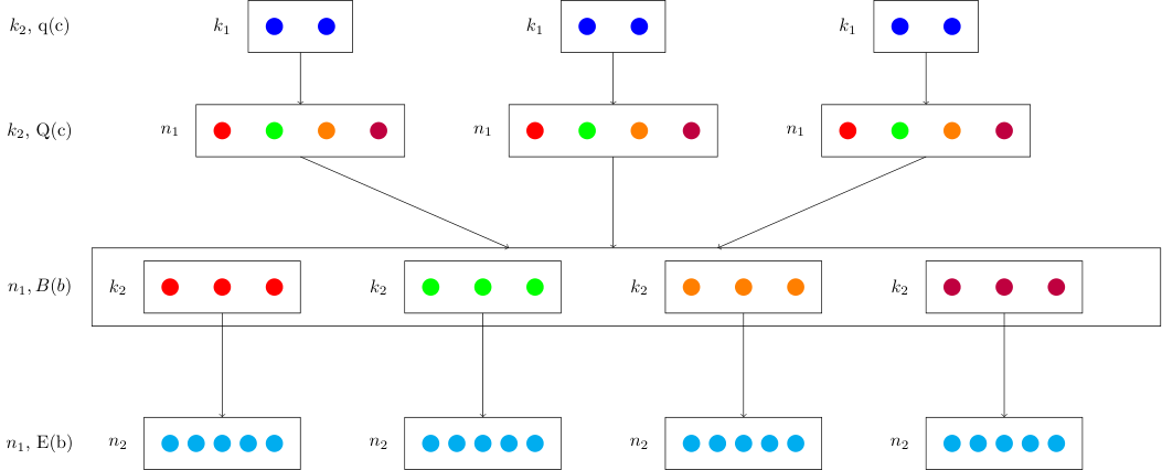
(1) The solution is to start with $k_2$ blocks of $k_1$ qubits each, which we will label as q(c), for $c=1,\dots,k_2$. So our initial state will be $$\ket{\Psi} = \ket{\psi^0}_{k_1} \otimes \ket{\psi^1}_{k_1} \otimes \cdots \otimes \ket{\psi^{k_2-1}}_{k_1},$$ where there are $k_2$ terms in the product. We have a total of $k_2k_1$ qubits. Note that this steps means we have given up on the ability to encode an unknown quantum state, for which we only have one copy. However, for quantum computational algorithms, we rarely start with an unknown state, so this is a not a big impediment.

(2) Next, we encode each block $q(c)$ using $C_1$ into a block $Q(c)$ of $n_2$ qubits. We obtain $$\ket{\Psi} \stackrel{C_1}{\to} \ket{\bar\Psi} = \ket{\bar\psi^0}_{n_1} \otimes \ket{\bar\psi^1}_{n_1} \otimes \cdots \otimes \ket{\bar\psi^{k_2-1}}_{n_1},$$ which has a total of $k_2n_1$ qubits.

(3) For the next step, we will need to rearrange the qubits. We are going to pick the first qubit in each $Q(c)$ and make that one block, take the second qubit in each $Q(c)$ and make those a block, and so on. Each new block will be called $B(b)$. Since, there are $k_2$ many $Q(c)$ blocks, each block $B(b)$ will of size $k_2$ as well, And because the size of $Q(c)$ is $n_1$, there will be $n_1$ many $B(b)$ blocks, with $b=0,\dots,n_1-1$.

To make this explicit, we operate on the states we created above. First, we expand one term in the product above in some basis to obtain $$\ket{\bar\psi^j}_{n_1} = \sum_{\lambda_i = 0,1}\alpha_\lambda\ket{\lambda_0^j\lambda_1^j\cdots\lambda^j_{n_1-1}}_{n_1}.$$ Then, $$\ket{\bar\Psi} = \sum_{\lambda^0_i = 0,1}\alpha_\lambda^0\ket{\lambda^0_0\lambda^0_1\cdots\lambda^0_{n_1-1}}_{n_1} \otimes \cdots \otimes \sum_{\lambda^{k_2-1}_i = 0,1}\alpha_\lambda^{k_2-1}\ket{\lambda^{k_2-1}_0\lambda^{k_2-1}_1\cdots\lambda^{k_2-1}_{n_1-1}}_{n_1}.$$ We can now rearrange these to obtain, $$\ket{\bar\Psi} = \sum_{\lambda^0_i,\dots,\lambda^{k_2-1}= 0,1}\alpha_\lambda^0\cdots\alpha_\lambda^{k_2-1} \ket{\lambda^0_0\lambda^1_0\cdots \lambda^{k_2-1}_0}_{k_2} \otimes \cdots \otimes \ket{\lambda^0_{n_2-1}\lambda^1_{n_2-1}\cdots \lambda^{k_2-1}_{n_2-1}}_{k_2}.$$ To summarize, this state has $n_1$ blocks of size $k_2$ for a total of $n_1k_2$ qubits.

(4) We can now encode each block using $C_2$. Hence, $$\ket{\bar\Psi} \stackrel{C_2}{\to} \ket{\bar{\bar\Psi}} = \sum_{\lambda^0_i,\dots,\lambda^{k_2-1}= 0,1}\alpha_\lambda^0\cdots\alpha_\lambda^{k_2-1} \ket{\overline{\lambda^0_0\lambda^1_0\cdots \lambda^{k_2-1}_0}}_{n_2} \otimes \cdots \otimes \ket{\overline{\lambda^0_{n_2-1}\lambda^1_{n_2-1}\cdots \lambda^{k_2-1}_{n_2-1}}}_{n_2}.$$ This state now has $n_1$ blocks $E(b)$ of size $n_2$, for a total of $n_1n_2$ qubits.

In summary, this concatenated code encodes $k=k_1k_2$ qubits into $n=n_1n_2$ qubits.

Obtaining the generators

We are now going to determine the generators of the final encoded state. Note, that we need a total of $n_1n_2-k_1k_2$ generators.

(1) As before, the generators of $C_2$ must by definition stabilize the state of each block $E(b)$, $$g^2_l\ket{\overline{\lambda^0_0\lambda^1_0\cdots \lambda^{k_2-1}_0}}_{n_2} = \ket{\overline{\lambda^0_0\lambda^1_0\cdots \lambda^{k_2-1}_0}}_{n_2}.$$

Hence, we assign a copy of all generators $g^2_l$ for each block $E(b)$ to our collection. This means $n_1(n_2-k_2)$ generators. The algorithm is the same, except for the number of $E(b)$ blocks.

(2) The encoding of the $C_1$ generators is much more subtle. If $g^1_l$ is applied to a $Q(c)$ block, it stabilizes the state $\ket{\bar\psi}$. But in the subsequent re-ordering, $Q(c)$ is broken up. To start with an example, consider $g^1_l$ acting on $Q(0)$, $$g^l_1 = P_0 \otimes P_1 \otimes \cdots \otimes P_{n_1-1}.$$ Where do the qubits that these $P_i$ act on go after the re-ordering. Since, this is the $0$-th block, $P_i$ now acts on the $0$-th position in the $B(i)$ block. Subsequently, when we encode each $B(i)$ using $C_2$, each of the $P_i$ will map the the corresponding $0$-th logical operator. Meaning if $P_i=X$, then after encoding it should be $\bar{X}_0$. In the same way, if $g^1_l$ acts on $Q(c)$, then all its constitutive Pauli operators $P_i$ go to the $c$-th location in $B(i)$ and hence should be mapped to $\bar{P}_c$.

The algorithm for this is as follows:

# declare
# logical_xs
# logical_zs
# iterate over each block Q(c)
for c in range(k2):
    for each g:
        encoded_g = zeros((1,2*n))
        # now iterate over the qubits in g
        for i in range(n1):
            if g[i] and g[n+i]: #P_i is the Y operator
                # place the c-th encoded logical gate into the E(b) block in the encoded_g
                encoded_g[n2*i: n2*(i+1)] += logical_xs[c][:n2] + logical_zs[c][:n2]
                encoded_g[n + n2*i: n + n2*(i+1)] += logical_xs[c][n2:] + logical_zs[c][n2:]
            elif g[i]: # P_i is the X operator
                encoded_g[n2*i: n2*(i+1)] += logical_xs[c][:n2]
                encoded_g[n + n2*i: n + n2*(i+1)] += logical_xs[c][n2:]
            elif g[n+i] # P_i is the Z operator
                encoded_g[n2*i: n2*(i+1)] += logical_zs[i][:n2]
                encoded_g[n + n2*i: n + n2*(i+1)] += logical_zs[c][n2:] 

We can also reproduce the example from the book, in which $C_1=[[5,13]]$ and $C_2 = [[4,2,2]]$.

cd2 = stac.CommonCodes.generate_code('[[5,1,3]]')
concat_code = stac.ConcatCode((cd2, cd))
stac.print_paulis(concat_code.generator_matrix)

$\displaystyle XZZXIIIIIIIIIIIIIIII$

$\displaystyle YXXYIIIIIIIIIIIIIIII$

$\displaystyle IIIIXZZXIIIIIIIIIIII$

$\displaystyle IIIIYXXYIIIIIIIIIIII$

$\displaystyle IIIIIIIIXZZXIIIIIIII$

$\displaystyle IIIIIIIIYXXYIIIIIIII$

$\displaystyle IIIIIIIIIIIIXZZXIIII$

$\displaystyle IIIIIIIIIIIIYXXYIIII$

$\displaystyle IIIIIIIIIIIIIIIIXZZX$

$\displaystyle IIIIIIIIIIIIIIIIYXXY$

$\displaystyle XIYYYZYIYZYIXIYYIIII$

$\displaystyle IIIIXIYYYZYIYZYIXIYY$

$\displaystyle XIYYIIIIXIYYYZYIYZYI$

$\displaystyle YZYIXIYYIIIIXIYYYZYI$

$\displaystyle XIXZIXZZIXZZXIXZIIII$

$\displaystyle IIIIXIXZIXZZIXZZXIXZ$

$\displaystyle XIXZIIIIXIXZIXZZIXZZ$

$\displaystyle IXZZXIXZIIIIXIXZIXZZ$

Stac can just put the two algorithms together and concatenate an arbitrary number of codes.

concat_code = stac.ConcatCode((cd, cd2, cd2))
print(concat_code)

A [[100,2]] code

A final note about distance

The book shows that if $C_1$ has distance $d_1$ and $C_2$ has distance $d_2$, then the concatenated code $C$ has distance at least $d_1d_2$. We will look into this more next time.

[1] Gaitan, Frank, Quantum Error Correction and Fault Tolerant Quantum Computing (CRC Press, 2008).