A QLDPC decoder

In an error-correction code, once the syndromes have been measured, the next step is to infer the error that has occurred on the physical qubits. This is a decoding algorithm to be run on a classical computer. Today, I want to explore a particular decoding algorithm (Delfosse et al. 2021, Berent et al. 2022), as a working example for understanding decoding.

We should begin by first building up some mathematical details. We will also need some example codes. Our classical code $C$ will be the Hamming code, which has parity check matrix, $$H=\begin{pmatrix} 1 & 1 & 1 & 1 & 0 & 0 & 0 \\ 1 & 1 & 0 & 0 & 1 & 1 & 0 \\ 1 & 0 & 1 & 0 & 1 & 0 & 1 \\ \end{pmatrix}.$$ Here, $n$ bits (columns) are constrained by $m$ checks (rows).

Recall that codewords are represented by elements of $\mathbb{F}_2^n$, and for any codeword $x \in C$, we have the constraint $Hx = 0$. Binary vectors $e \in \mathbb{F}_2^n$ and $e \not\in C$ fail this constraint. We call such vectors (non-trivial) errors. The syndrome of the error is $\sigma(e) = He \in \mathbb{F}_2^m$.

import numpy as np

H = np.array([[1, 1, 1, 1, 0, 0, 0],
       [1, 1, 0, 0, 1, 1, 0],
       [1, 0, 1, 0, 1, 0, 1]])

# sample error
e = [1, 0, 0, 0, 0, 1, 0]

print("syndrome =", H@e % 2)

syndrome = [1 0 1]

Tanner graphs

One way of graphically visualizing a code is by creating a Tanner graph. Given code $C$, the tanner graph is $$T(C) = (V=V_D \cup V_C, E),$$ where $V_D$ is a set of vertices associated with the data qubits, and $V_C$ is a set of qubits associated with the parity checks. If the $i$-th data bit is involved in the $j$-th parity check, then there is an edge from $i$th vertex in $V_C$ to the $j$-th vertex in $V_D$.

The following two functions allow us to create and draw the Tanner graph of any classical code.

import networkx as nx
import matplotlib.pyplot as plt

def tanner_graph(H: np.ndarray):
    "Create tanner graph from a parity check matrix H."
    m, n = H.shape
    T = nx.Graph()

    T.H = H
    # nodes
    T.VD = [i for i in range(n)]
    T.VC = [-j-1 for j in range(m)]

    # add them, with positions
    for i, node in enumerate(T.VD):
        T.add_node(node, pos=(i-n/2, 0), label='$d_{'+str(i)+'}$')
    for j, node in enumerate(T.VC):
        T.add_node(node, pos=(j-m/2, 1), label='$c_{'+str(j)+'}$')

    # add checks to graph
    for j, check in enumerate(H):
        for i, v in enumerate(check):
            if v:
                T.add_edge(-j-1, i)

    return T

def draw_tanner_graph(T, highlight_vertices=None):
    "Draw the graph. highlight_vertices is a list of vertices to be colored."
    pl=nx.get_node_attributes(T,'pos')
    lbls = nx.get_node_attributes(T, 'label')

    nx.draw_networkx_nodes(T, pos=pl, nodelist=T.VD, node_shape='o')
    nx.draw_networkx_nodes(T, pos=pl, nodelist=T.VC, node_shape='s')
    nx.draw_networkx_labels(T, pos=pl, labels=lbls)

    nx.draw_networkx_edges(T, pos=pl)

    if highlight_vertices:
        nx.draw_networkx_nodes(T,
                               pos=pl,
                               nodelist=[int(v[1]) for v in highlight_vertices if v[0] == 'd'],
                               node_color='red',
                               node_shape='o')
        nx.draw_networkx_nodes(T,
                       pos=pl,
                       nodelist=[-int(v[1])-1 for v in highlight_vertices if v[0] == 'c'],
                       node_color='red',
                       node_shape='s')

    plt.axis('off');

# these four functions allow us to convert between 
# (s)tring names of vertices and (i)nteger names of vertices
def s2i(node):
    return int(node[1]) if node[0] == 'd' else -int(node[1])-1

def i2s(node):
    return f'd{node}' if node>=0 else f'c{-node-1}'

def ms2i(W: set):
    return set(map(s2i, W))

def mi2s(W: set):
    return set(map(i2s, W))

T = tanner_graph(H)
draw_tanner_graph(T)

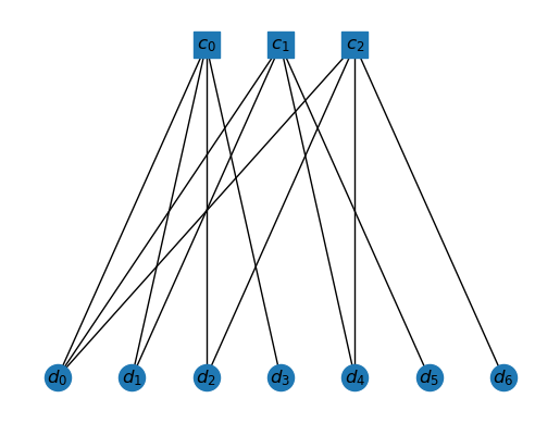
The operations of the code can be done using these graphs. For example, any vector in $\mathbf{F}_2^2$ can be assigned to the data vertices. Then a parity check corresponding to a check vertex is implemented by computing the parity of the data vertices connected to this check vertex.

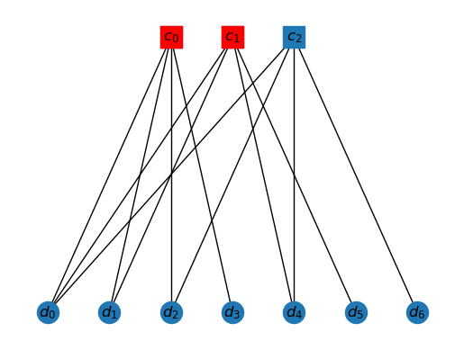
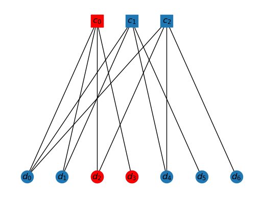
We can also specify the syndrome on the graph. A syndrome is the set of check qubits that light up. So, if error $d_1$ occurs, then $c_0$ and $c_1$ trigger. So the syndrome $\sigma(\{d_1\}) = \{c_0,c_1\}$ is shown as follows.

draw_tanner_graph(T, ['c0', 'c1'])

Some essential graph concepts

We will need some graph concepts that we should define. The first definition is quite straightforward.

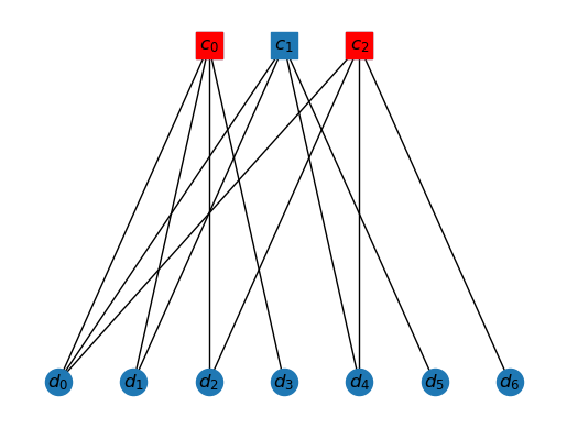
Given $G=(V,E)$ and given $v \in V$, the neighbors $N(v) \subseteq V$ of $v$ is the subset of vertices in $V$ that are connected by an edge to $v$.

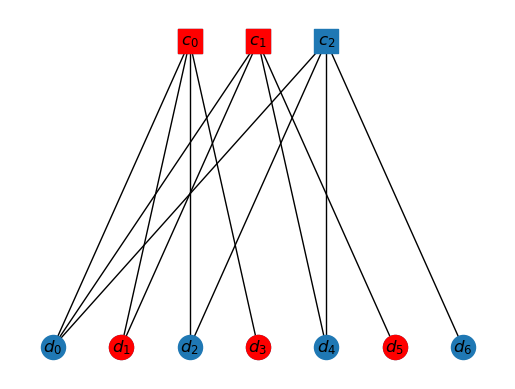
As an example, the neighbors of $d_2$ are given by

draw_tanner_graph(T, ['c0','c2'])

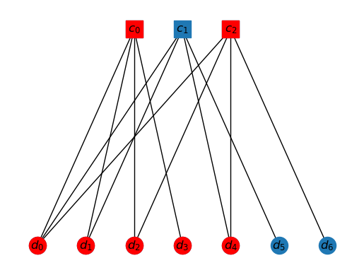
The next property is related to sets of vertices. The interior of a set of vertices is that subset of vertices who all have neighbors inside the interior. Basically, if edges are viewed as relationships between vertices, than the interior is those vertices which are only related to those inside the interior.

Given a subset of vertices $W \subseteq V$, the interior $Int(W)$ of $W$ has vertices $v \in Int(W)$ if and only if $N(v) \subseteq Int(W)$.

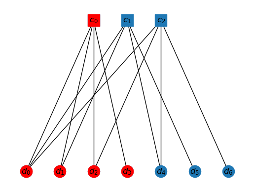
Consider the following subset of vertices

Vs = set(['c0', 'c2', 'd0', 'd1', 'd2', 'd3', 'd4'])
draw_tanner_graph(T, Vs)

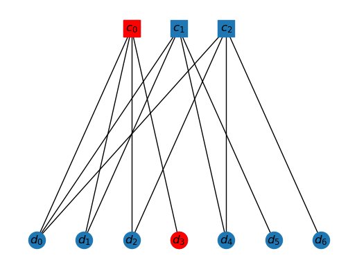
This set has interior as follows.

def interior(T, W):
    "Determine interior of vertex subset W of Tanner graph T."
    IntW = set()
    for v in W:
        if set(nx.neighbors(T,v)).issubset(W):
            IntW.add(v)
    return IntW

draw_tanner_graph(T, mi2s(interior(T, ms2i(Vs))))

Quantum CSS codes

A quantum CSS code is made of two parity check matrices (PCMs). The $X$-checks are $H_X \in \mathbb{F}_2^{m\times n}$ and the $Z$-checks are $H_Z \in \mathbb{F}_2^{l \times n}$, with the constraint that $$H_XH_Z^T = 0.$$

Now, there are two types of errors possible, bit-fip errors and phase-flip errors. So an error is a vector $e = (e_X,e_Z) \in \mathbb{F}_2^n \times \mathbb{F}_2^n$. The syndrome for bit-flip errors is $\sigma(e_X) = H_Xe_X \in \mathbb{F}_2^m$ and the syndrome for phase-flip errors is $\sigma(e_Z) = H_Ze_Z \mathbb{F}_2^l$.

The beauty of CSS codes is that bit-flip and phase-flip errors are corrected separately. So, we don't really have to generalize the Tanner graphs to CSS codes. These are dealt with one by one in the decoding algorithm.

QLDPC decoder

The decoder is broken into an $X$-detector and a $Z$-detector, which are identical. The input of the $X$-detector is the syndrome $\sigma(e_X)$. The goal of the detector is to output an error $\tilde{e}_X$ such that $\sigma(\tilde{e}_X) = \sigma(e_X)$. Similarly for the $Z$-decoder. Therefore, in the following we will just refer to error $e$, rather than $e_X$ or $e_Z$

One definition first, before we discuss further.

A cluster is a subset of vertices of the Tanner graph.

The algorithm has two main steps sandwiched between two minor ones.

1. Assign each lit-up check vertex to its own cluster.
2. Initially, all these clusters will be "invalid" (explained below). Iteratively, each cluster is grown by adding its neighbors, until all clusters are valid. As these clusters grow, some might merge. At the end, each vertex in $T$ will be part of exactly one cluster or no cluster at all.
3. Each cluster will have some data vertices and some check vertices. For each cluster, separately, determine an estimated error (values of data vertices) that are consistent with the syndrome values of the check vertices.
4. Collect the estimated errors for the clusters into one estimated error.

Let us now now discuss the validity of clusters and how to determine the estimate for each cluster.

Valid and invalid clusters

Given a syndrome $\sigma(e)$, a valid cluster is defined by the following definition.

Let $K^i$ be a cluster. $K^i$ is valid if and only if there exists an estimated error (a set of data vertices) $\tilde{e}^i \subseteq V_D \cap Int(K^i)$ such that $\sigma(\tilde{e}^i) = \sigma(e) \cap K^i$.

That is a mouthful, so let us break this down. We already understand what $Int(K^i)$ is. Then $V_D \cap Int(K^i)$ is just the data vertices in the interior of $K^i$. Next, $\sigma(e) \cap K_i$ is the triggered check vertices that are also in $K_i$.

So, given a cluster $K^i$ and error $e$, we only consider the data vertices inside the cluster. If we light some of them up, we get a partial candidate error $\tilde{e}^i$. If we compute the corresponding syndrome $\sigma(\tilde{e}^i)$ and it turns out that the check vertices that light up are exactly those in $\sigma(e) \cap K^i$, then the cluster is valid. Let's look at an example.

Consider the following situation. Let $\sigma(e) = \{c_0\}$, and let $K^0$ be the following.

K0 = ['c0', 'd0', 'd1','d2', 'd3']
draw_tanner_graph(T, K0)

The interior of this cluster is just $\{d_3, c_0\}$, as all others have neighbor outside the cluster.

draw_tanner_graph(T, mi2s(interior(T, ms2i(K0))))

This is quite a simple problem. There is only one vertex in $V_D \cap Int(K^i)$, which is $d_3$. If we light this up, then it will in turn trigger $c_0$ only, i.e. $\sigma(\{d_3\}) = \{c_0\}$. Moreover, $\sigma(x) \cap K^i = \{c_0\}$. So, indeed our assignment $\sigma(\{d_3\}) = \sigma(x) \cap K^i$. Hence, this is a valid cluster.

Here is another example. Drawn is in the interior of the cluster K1. Can you identify the solution?

K1 = ['c0', 'c1', 'd0', 'd1','d2', 'd3','d4','d5']
draw_tanner_graph(T, mi2s(interior(T, ms2i(K1))))

In general, we have a linear algebra problem. Let $H_{\sigma(x) \cap K^i}$ be the submatrix of $H$ created by choosing the checks that are in the cluster. In the example above, this will just be the first check. Let $\sigma(e)_{V_D \cap Int(K^i)}$ be the submatrix (subvector) of the syndrome which only involves the elements corresponding to the checks that are in the cluster. In the example above, this is again the first element of the syndrome vector. Then, we have the relation, $$H_{\sigma(x) \cap K^i}\tilde{e} = \sigma(e)_{V_D \cap Int(K^i)}$$ So

1. To check if a cluster is valid, all we have to check is if a solution exists to the above linear problem.
2. To determine $\tilde{e}$, we solve this linear system.

Hence, we want to write two functions, that take in a cluster and a syndrome as input. One determines if it is valid or invalid, and other outputs the error estimate $\tilde{e}$ that satisfies a valid cluster.

First, we need functions to deal with finite field linear algebra problems, since such functions don't exist in standard libraries.

import numpy as np
import galois

def solvable_system(A,b):
    "Determines if there is a solution to Ax=b."
    A_rank = np.linalg.matrix_rank(A)

    # create augmented matrix
    Ab = np.hstack((A, np.atleast_2d(b).T))

    # Must be true for solutions to be consistent
    return A_rank == np.linalg.matrix_rank(Ab)

def solve_underdetermined_system(A, b):
    "Returns a random solution to Ax=b."
    n_vars = A.shape[1]
    A_rank = np.linalg.matrix_rank(A)

    # create augmented matrix
    Ab = np.hstack((A, np.atleast_2d(b).T))

    # Must be true for solutions to be consistent
    if A_rank != np.linalg.matrix_rank(Ab):
        raise Exception("No solution exists.")

    # reduce the system
    Abrr = Ab.row_reduce()

    # additionally need form in which the identity
    # is moved all the way to the left. Do some
    # column swaps to achieve this.
    swaps = []
    for i in range(min(Abrr.shape)):
        if Abrr[i,i] == 0:
            for j in range(i+1,n_vars):
                if Abrr[i,j] == 1:
                    Abrr[:, [i,j]] = Abrr[:, [j,i]]
                    swaps.append((i,j))
                    break

    # randomly generate some independent variables
    n_ind = n_vars - A_rank
    ind_vars = A.Random(n_ind)

    # compute dependent variables using reduced system and dep vars
    dep_vars = -Abrr[:A_rank,A_rank:n_vars]@ind_vars + Abrr[:A_rank,-1]

    # x is just concatenation of the two
    x = np.hstack((dep_vars, ind_vars))

    # swap the entries of x according to the column swaps earlier
    # to get the solution to the original system.
    for s in reversed(swaps):
        x[s[0]], x[s[1]] = x[s[1]], x[s[0]]

    return x

Here is the function to determine if a cluster is valid. An example is included, where the cluster is equal to its interior. Make sure you understand why it is valid.

syndrome = [1,1,0]
cluster = ms2i(['c0', 'c1', 'd1'])

def is_valid_cluster(T, syndrome, cluster):
    "Given a syndrome and cluster, determines if is is valid."

    cluster_interior = interior(T, cluster)

    data_qubits_in_interior = sorted([i for i in cluster_interior if i>=0])
    check_qubits_in_cluster = sorted([-i-1 for i in cluster if i<0])

    GF = galois.GF(2)
    A = GF(T.H[check_qubits_in_cluster][:,data_qubits_in_interior])
    b = GF([syndrome[i] for i in check_qubits_in_cluster])

    solved = solvable_system(A,b)

    return solved

is_valid_cluster(T, syndrome, cluster)

True

To find a valid correction, we solve the problem.

def find_valid_correction(T, syndrome, cluster):

    cluster_interior = interior(T, cluster)

    data_qubits_in_interior = sorted([i for i in cluster_interior if i>=0])
    check_qubits_in_cluster = sorted([-i-1 for i in cluster if i<0])

    GF = galois.GF(2)
    A = GF(T.H[check_qubits_in_cluster][:,data_qubits_in_interior])
    b = GF([syndrome[i] for i in check_qubits_in_cluster]) 

    sol = solve_underdetermined_system(A,b)

    return sol, data_qubits_in_interior

A nice function to determine the neighbors of a cluster.

def cluster_neighbors(T, cluster):
    nbrs = set()
    for v in cluster:
        nbrs.update(set(nx.neighbors(T,v)))
    return nbrs

And here is our decoder. If you read the original papers, you will realize that they study multiple ways of choosing which clusters to grow in each iteration. I have just chosen one method, which does not seem to correspond to any of the methods they choose. The decoder is also not at all very efficiently written, but it should work.

def ldpc_decoder(T, syndrome):

    n = len(T.VD)

    # assign each syndrome to its own cluster
    K = [set([-i-1]) for i,s in enumerate(syndrome) if s]

    # grow clusters till all are valid
    while True:
        # if during the loop below some clusters are
        # merged, then we restart the loop
        K_updated = False
        # When clusters are merged, then later need to
        # delete the one that was added to the other.
        to_delete = []
        # print(f"Restarting {K}")
        for i, Ki in enumerate(K):
            # print(f'K{i} = {Ki}')
            if not is_valid_cluster(T, syndrome, Ki):
                nbrs = cluster_neighbors(T, Ki)
                Ki.update(nbrs)
                # print(f'K{i} with nbrs = {Ki}')
                # for loop to check if clusters need to
                # be merged with this newly grown one
                for j, Kj in enumerate(K):
                    if j < i and (not nbrs.isdisjoint(Kj)):
                        Kj.update(Ki)
                        # print(f'K{j} with K{i} = {Kj}')
                        to_delete.append(i)
                        K_updated = True
                    elif j > i and (not nbrs.isdisjoint(Kj)):
                        Ki.update(Kj)
                        # print(f'K{i} with K{j} = {Ki}')
                        to_delete.append(j)
                        K_updated = True
                if K_updated:
                    break
        for i in reversed(to_delete):
            K.pop(i)
        if K_updated == False:
            break

    # determine error estimate using valid clusters
    e_estimate = np.array([0]*n)
    for i, Ki in enumerate(K):
        correction, correction_data_qubits = find_valid_correction(T, syndrome, Ki)
        e_estimate[correction_data_qubits] = correction

    return e_estimate

syndrome = [1,1,0]
e_estimate = ldpc_decoder(T, syndrome)
print(f'{e_estimate=}')
print(f'Correct estimate? {all((H@e_estimate %2) == syndrome)}')

e_estimate=array([0, 0, 0, 1, 0, 1, 0])
Correct estimate? True

Testing on real qldpc codes

We import a simple qldpc code, with the help of this guide.

from bposd.hgp import hgp
from random import randint
import time

HL = np.array([[1, 1, 0, 0, 1, 1, 0, 0, 0, 0, 0, 0, 0, 0, 0, 0],
            [0, 0, 1, 0, 0, 0, 1, 1, 0, 0, 0, 0, 1, 0, 0, 0],
            [0, 0, 0, 1, 1, 0, 1, 0, 0, 0, 0, 0, 0, 1, 0, 0],
            [0, 0, 0, 0, 0, 1, 0, 0, 1, 1, 0, 0, 0, 0, 0, 1],
            [0, 1, 0, 0, 0, 0, 0, 1, 1, 0, 0, 1, 0, 0, 0, 0],
            [0, 0, 0, 0, 0, 0, 0, 0, 1, 0, 0, 0, 1, 1, 1, 0],
            [1, 0, 0, 0, 0, 0, 0, 1, 0, 0, 0, 0, 0, 1, 0, 1],
            [0, 0, 0, 1, 0, 1, 0, 0, 0, 0, 1, 0, 1, 0, 0, 0],
            [0, 0, 1, 1, 0, 0, 0, 0, 0, 0, 0, 1, 0, 0, 0, 1],
            [0, 0, 0, 0, 1, 0, 0, 0, 0, 1, 1, 1, 0, 0, 0, 0],
            [0, 1, 0, 0, 0, 0, 1, 0, 0, 0, 1, 0, 0, 0, 1, 0],
            [1, 0, 1, 0, 0, 0, 0, 0, 0, 1, 0, 0, 0, 0, 1, 0]])
qcode=hgp(HL,HL,compute_distance=True)
qcode.test()
Hx = qcode.hx
Tx = tanner_graph(Hx)

, (4,7)-[[400,16,6]]
 -Block dimensions: Pass
 -PCMs commute hz@hx.T==0: Pass
 -PCMs commute hx@hz.T==0: Pass
 -lx \in ker{hz} AND lz \in ker{hx}: Pass
 -lx and lz anticommute: Pass
 - is a valid CSS code w/ params (4,7)-[[400,16,6]]

This is a distance 6 code, so it can surely correct 2 errors. Since, the code is CSS and the decoder works separately on $X$ and $Z$ syndromes, we only really need to test this on one of the parts.

# random error with one or two flip only
x_error = [0]*qcode.N
x_error[randint(0,qcode.N-1)] = 1
if randint(0,1):
    x_error[randint(0,qcode.N-1)] = 1

# the corresponding syndrome
syndrome = Hx@x_error %2
print(f'{syndrome=}')

start = time.perf_counter()
e_estimate = ldpc_decoder(Tx, syndrome)
end=time.perf_counter()

print(f'{e_estimate=}')
print(f'Estimate reproduces syndrome? {all((Hx@e_estimate %2) == syndrome)}')
print(f'Estimate = original error? {all(e_estimate == x_error)}')
print(f"Completed in {end - start:0.4f} seconds")

syndrome=array([0, 0, 0, 0, 0, 0, 0, 0, 0, 0, 0, 0, 0, 0, 0, 1, 0, 0, 0, 0, 0, 0,
       0, 0, 0, 0, 0, 0, 0, 0, 0, 0, 0, 0, 0, 0, 0, 0, 0, 0, 0, 0, 0, 0,
       0, 0, 0, 0, 0, 0, 0, 0, 0, 0, 0, 0, 0, 0, 0, 0, 0, 0, 0, 1, 0, 0,
       0, 0, 0, 0, 0, 0, 0, 0, 0, 0, 0, 0, 0, 0, 0, 0, 0, 0, 0, 0, 0, 0,
       0, 0, 0, 0, 0, 0, 0, 0, 0, 0, 0, 0, 0, 0, 0, 0, 0, 0, 0, 0, 0, 0,
       0, 0, 0, 0, 0, 0, 0, 0, 0, 0, 0, 0, 0, 0, 0, 0, 0, 1, 0, 0, 0, 0,
       0, 0, 0, 0, 0, 0, 0, 0, 0, 0, 0, 0, 0, 0, 0, 0, 0, 0, 0, 0, 0, 0,
       0, 0, 0, 0, 0, 0, 0, 0, 0, 0, 0, 0, 0, 0, 0, 0, 0, 0, 0, 0, 0, 0,
       0, 0, 0, 0, 0, 0, 0, 0, 0, 0, 0, 0, 0, 0, 0, 0])
e_estimate=array([0, 0, 0, 0, 0, 0, 0, 0, 0, 0, 0, 0, 0, 0, 0, 0, 0, 0, 0, 0, 0, 0,
       0, 0, 0, 0, 0, 0, 0, 0, 0, 0, 0, 0, 0, 0, 0, 0, 0, 0, 0, 0, 0, 0,
       0, 0, 0, 0, 0, 0, 0, 0, 0, 0, 0, 0, 0, 0, 0, 0, 0, 0, 0, 0, 0, 0,
       0, 0, 0, 0, 0, 0, 0, 0, 0, 0, 0, 0, 0, 0, 0, 0, 0, 0, 0, 0, 0, 0,
       0, 0, 0, 0, 0, 0, 0, 1, 0, 0, 0, 0, 0, 0, 0, 0, 0, 0, 0, 0, 0, 0,
       0, 0, 0, 0, 0, 0, 0, 0, 0, 0, 0, 0, 0, 0, 0, 0, 0, 0, 0, 0, 0, 0,
       0, 0, 0, 0, 0, 0, 0, 0, 0, 0, 0, 0, 0, 0, 0, 0, 0, 0, 0, 0, 0, 0,
       0, 0, 0, 0, 0, 0, 0, 0, 0, 0, 0, 0, 0, 0, 0, 0, 0, 0, 0, 0, 0, 0,
       0, 0, 0, 0, 0, 0, 0, 0, 0, 0, 0, 0, 0, 0, 0, 0, 0, 0, 0, 0, 0, 0,
       0, 0, 0, 0, 0, 0, 0, 0, 0, 0, 0, 0, 0, 0, 0, 0, 0, 0, 0, 0, 0, 0,
       0, 0, 0, 0, 0, 0, 0, 0, 0, 0, 0, 0, 0, 0, 0, 0, 0, 0, 0, 0, 0, 0,
       0, 0, 0, 0, 0, 0, 0, 0, 0, 0, 0, 0, 0, 0, 0, 0, 0, 0, 0, 0, 0, 0,
       0, 0, 0, 0, 0, 0, 0, 0, 0, 0, 0, 0, 0, 0, 0, 0, 0, 0, 0, 0, 0, 0,
       0, 0, 0, 0, 0, 0, 0, 0, 0, 0, 0, 0, 0, 0, 0, 0, 0, 0, 0, 0, 0, 0,
       0, 0, 0, 0, 0, 0, 0, 0, 0, 0, 0, 0, 0, 0, 0, 0, 0, 0, 0, 0, 0, 0,
       0, 0, 0, 0, 0, 0, 0, 0, 0, 0, 0, 0, 0, 0, 0, 0, 0, 0, 0, 0, 0, 0,
       0, 0, 0, 0, 0, 0, 0, 0, 0, 0, 0, 0, 0, 0, 0, 0, 0, 0, 0, 0, 0, 0,
       0, 0, 0, 0, 0, 0, 0, 0, 0, 0, 0, 0, 0, 0, 0, 0, 0, 0, 0, 0, 0, 0,
       0, 0, 0, 0])
Estimate reproduces syndrome? True
Estimate = original error? True
Completed in 0.0257 seconds

There you have it. A working decoder. If you run this many times, you will find that sometimes it fails. By failure, I mean that it finds a high weight error (in this case, much larger than 2), that gives the correct syndrome but if used will distort the code state further. The reason for this is that there are multiple solutions to the linear algebra problem, and sometimes the a very "high weight" solution is discovered.

Let us estimate the percentage of failure.

runs = 10**4
n_incorrect = 0

for i in range(runs):
    x_error = [0]*qcode.N
    x_error[randint(0,qcode.N-1)] = 1
    if randint(0,1):
        x_error[randint(0,qcode.N-1)] = 1

    syndrome = Hx@x_error %2
    e_estimate = ldpc_decoder(Tx, syndrome)

    if not all(e_estimate == x_error):
        n_incorrect += 1

print(f'Fraction incorrect {n_incorrect/runs:0.2f}')

Fraction incorrect 0.08

As you see about 8% of the runs failed, which is quite a large error.